What is an AQL (Acceptable Quality Limit) and How to Use It?

In mass production, inspecting 100% of goods is often cost-prohibitive and operationally inefficient. To balance quality assurance with speed, supply chain professionals rely on the Acceptance Quality Limit (AQL). Defined by the international standard ISO 2859-1, AQL provides a statistical framework for accepting or rejecting a production batch based on random sampling. This guide outlines the core mechanics of AQL, including defect classification, sampling levels, and the practical application of standard inspection tables to mitigate risk in global sourcing.

Core Concepts and Definitions of Acceptance Quality Limit (AQL)

The Acceptable Quality Limit (AQL) is a quality control parameter defined in ISO 2859-1 as the “worst tolerable” quality level for a product lot. This metric indicates the maximum number of defective items acceptable during a random sampling inspection. AQL establishes a predetermined standard to help organizations manage quality and mitigate the risk of shipping faulty products. Inspectors express this limit as a percentage or ratio of defective units to the total lot quantity. In 2008, the terminology changed from “acceptable quality level” to “acceptable quality limit” to reflect its function as a boundary.

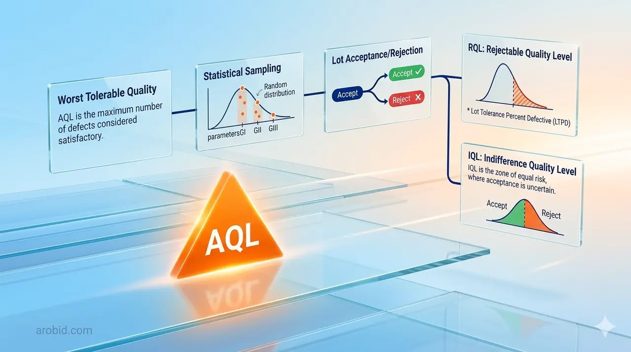
In practice, AQL is used in statistical sampling plans as an alternative to 100% inspection. Instead of checking every unit in a production batch, a defined sample is drawn at random. If the number of defective units in this sample is at or below the limit associated with the selected AQL, the lot is accepted. If the count exceeds that limit, the lot is rejected. When a lot is rejected, manufacturers typically review and adjust the production process to identify and correct the causes of nonconformance.

Two other metrics frame AQL:

• Rejectable Quality Level (RQL): Also known as Lot Tolerance Percent Defective (LTPD), this defines the threshold for an unacceptable number of defects.
• Indifference Quality Level (IQL): This level sits between AQL and RQL, representing a quality level that is neither explicitly good nor bad.

In organizations that apply Six Sigma or similar quality management systems, AQL is often used as one of the parameters in lot acceptance decisions. It links the statistical design of sampling plans with operational requirements on defect rates and helps align inspection activities with defined quality targets and supplier performance criteria.

The Role of AQL in Quality Management

AQL provides a standardized, data-driven approach to quality control. It establishes enforceable limits on acceptable defects, ensuring products align with customer expectations. This consistency minimizes the risk of end-users receiving substandard goods, which supports customer trust.

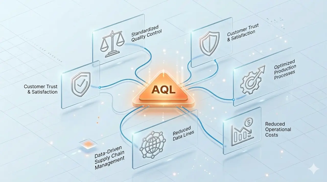
For manufacturers, AQL sets clear guidelines for internal processes. Teams can identify and correct production issues before shipment. This reduces financial risks associated with product recalls and customer complaints.

In supply chain management, organizations use AQL to monitor supplier performance against contractual standards. This data supports decisions regarding supplier partnerships. Additionally, replacing 100% inspection with statistical sampling reduces operational costs and resource allocation.

Key Benefits of Implementing AQL

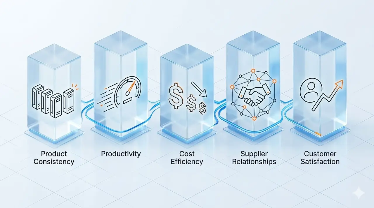
• Customer Satisfaction: Delivering products that meet pre-defined standards reduces the rate of defects reaching the end-user. This minimizes returns and supports customer retention.
• Cost Efficiency: Statistical sampling replaces 100% inspection, which lowers direct labor costs. Additionally, identifying defects early reduces material waste and scrap.
• Productivity: Early detection prevents faulty items from moving further down the production line. This minimizes rework and maintains production speed.
• Supplier Relationships: AQL provides quantifiable quality requirements. This clarity allows buyers to objectively evaluate supplier performance based on agreed metrics rather than subjective assessment.
• Product Consistency: Applying a uniform standard ensures consistency across different production batches, regardless of the manufacturing date or location.

Categorization of Defects in AQL

ISO 2859, Sampling procedures and tables for inspection by attributes, groups defects into three severity levels. This structure helps organizations prioritize risk and set clear acceptance limits.

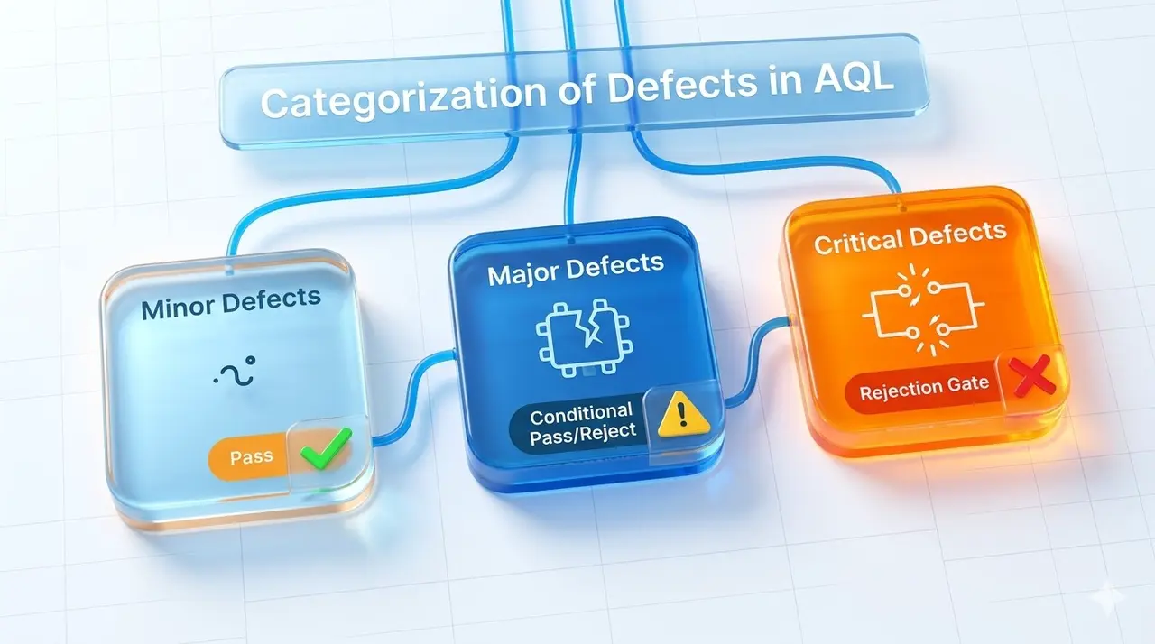
Critical Defects

Critical defects render the product unsafe or hazardous to the end-user. They also include deviations that violate mandatory regulations. Due to liability risks and safety concerns, the default AQL for this category is 0%. Finding a single critical defect typically results in the rejection of the entire batch.

Example: A sharp object (needle) found inside a garment.

Major Defects

Major defects affect the product’s functionality or significantly impact its appearance, leading to a likely failure or customer return. While not unsafe, these defects render the product commercially unacceptable. For consumer goods, the standard industry AQL is 2.5%.

Example: A battery in an electronic device that fails to charge.

Minor Defects

Minor defects are cosmetic deviations or workmanship issues that do not affect the product’s intended function or structural integrity. The end-user may still accept the product despite these imperfections. The standard AQL for minor defects is typically set at 4.0%.

Example: A small scratch on the surface of a cabinet.

AQL Standards Across Different Industries

AQL standards are not universal; they vary based on regulatory requirements and risk assessments. Organizations define these limits by weighing the cost of rigorous inspection against the potential liability of product failure.

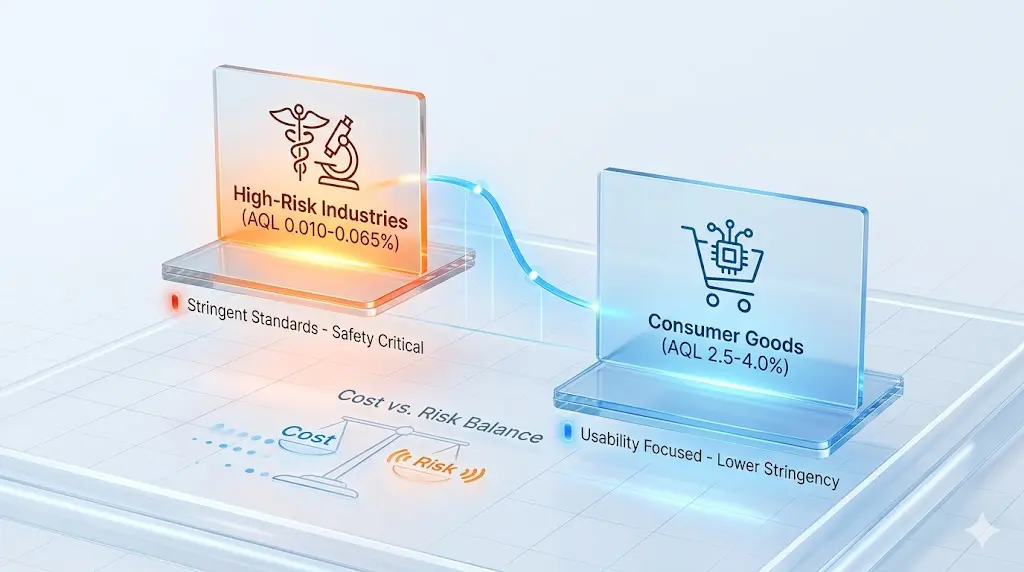
High-Risk Industries (Medical & Pharmaceuticals)

In sectors where product failure impacts user safety, regulations mandate stringent acceptance limits. For medical devices and pharmaceuticals, the allowable defect rate is extremely low to comply with safety standards (e.g., FDA 21 CFR Part 820). Common AQLs for critical features in these industries range from 0.010% to 0.065%.

Consumer Goods (Apparel & Electronics)

For products where defects affect usability rather than safety, inspection standards are less stringent. The global sourcing industry typically adopts AQL 2.5% (Major defects) and AQL 4.0% (Minor defects) as the baseline for apparel, electronics, and household goods.

Cost vs. Risk Balance

Tighter AQLs (lower percentages) require larger sample sizes, increasing inspection time and labor costs. Companies apply tighter standards only when the financial impact of a recall or the risk of regulatory non-compliance outweighs the operational cost of inspection.

The AQL Sampling Process

The strategic value of AQL random sampling lies in its ability to provide a statistically valid assessment of a lot’s quality without the prohibitive time and expense of a 100% inspection. The process is governed by a set of preliminary metrics that must be established to guide the final decision of whether to approve or disapprove of a production batch.

Inspection Levels

AQL sampling validates lot quality using statistical probabilities rather than 100% inspection. The process relies on Inspection Levels defined in ISO 2859-1, which determine the relationship between the lot size and the sample size.

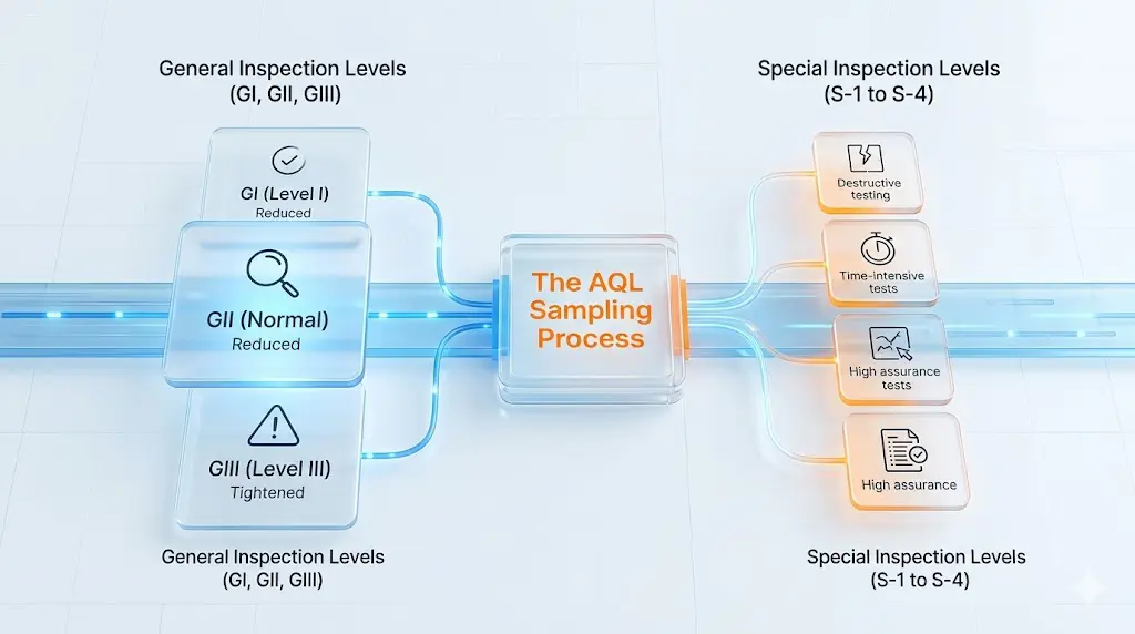
General Inspection Levels (GI, GII, GIII)

These levels dictate the sample size for visual and functional inspections of the primary product.

• Level II (Normal): The industry standard default. Unless specified otherwise, inspection protocols utilize Level II. It offers the standard balance between producer risk and consumer risk.
• Level I: Used by suppliers with a proven track record of quality. It typically requires a sample size approximately 40% of Level II, reducing inspection time and cost.
• Level III: Applied to high-risk lots or new suppliers. It requires a sample size approximately 160% of Level II, increasing the probability of detecting defects.

Special Inspection Levels (S-1 to S-4)

Special levels utilize very small sample sizes and are reserved for tests where large samples are impractical. Common applications include:

• Destructive Testing: Tests that damage the product (e.g., fabric gsm check, drop tests, seam strength).
• Time-Intensive Checks: Procedures taking significant time per unit (e.g., full assembly of complex furniture).
• High Assurance: Situations where the cost of inspection outweighs the risk of passing a defect.

Difference Between S-1, S-2, S-3, and S-4 on the AQL Table

The four Special Inspection Levels represent a hierarchy of sample size and discrimination power. Moving from S-1 to S-4, the sample size increases, providing greater statistical confidence but requiring more time and resources.

	S-1: The Minimal Check	S-2: Basic Physical Verification	S-3: Functional & Destructive Testing (Industry Standard)	S-4: High-Precision Special Testing
Sample Size	Smallest (Lowest discrimination)	Small (> S-1)	Moderate (Industry Default)	Largest (Approaches GI Level I)
Application	Administrative and packaging verification where internal product quality is not the focus.	Verification of non-critical physical characteristics, often consistent due to automated manufacturing.	Functional and destructive testing. Balances statistical validity with practical limits (minimizing product destruction).	High-precision testing. Used when specific performance metrics are critical, but full General Inspection is impractical.
Typical Use Cases	Checking shipping label barcodes. Verifying carton markings. Counting items per master carton.	Measuring shipping carton dimensions. Checking gross weight. Verifying material thickness.	Carton drop tests. Garment seam strength (pull test). Full assembly of furniture items. Adhesive bonding tests.	Reliability testing (e.g., Hi-pot test for electronics). Water resistance testing (watches/devices). Laboratory chemical analysis.

Note: S-3 is the standard default level used by most third-party inspection agencies (e.g., QIMA, Intertek) for on-site functionality checks and carton drop tests unless the buyer specifies otherwise.

Sampling Methods

ISO 2859-1 outlines three primary sampling plans, each balancing administrative cost against statistical efficiency.

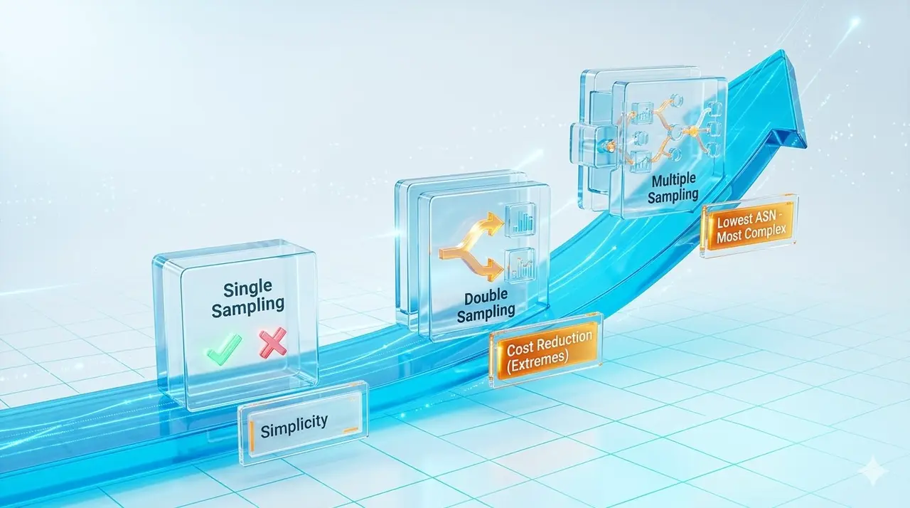
Single Sampling

In this widely adopted plan, inspectors draw one random sample of size n from the lot. The decision involves a single Acceptance number (Ac) and Rejection number (Re).

• If defects ≤ Ac: Accept the lot.
• If defects ≥ Re: Reject the lot.
• Advantage: Simplicity and ease of administration

Double Sampling

This method allows for a smaller initial sample size. If the first sample yields a defect count between the Ac and Re (an inconclusive range), inspectors draw a second sample. The final decision relies on the cumulative number of defects from both samples.

Advantage: Can lower total inspection costs for lots of very good or very poor quality (where the decision is made on the first small sample).

Multiple Sampling

Similar to Double Sampling but extends up to seven rounds of sampling. After each step, the cumulative defect count determines whether to accept, reject, or continue to the next sample.

Advantage: Lowest average sample size (Average Sample Number – ASN) but most complex to administer administratively.

Note: “Sequential Sampling” mentioned in statistical theory is functionally similar to Multiple Sampling in the context of ISO 2859, usually analyzing groups rather than single units to maintain efficiency.

Relationship Between AQL and Sampling

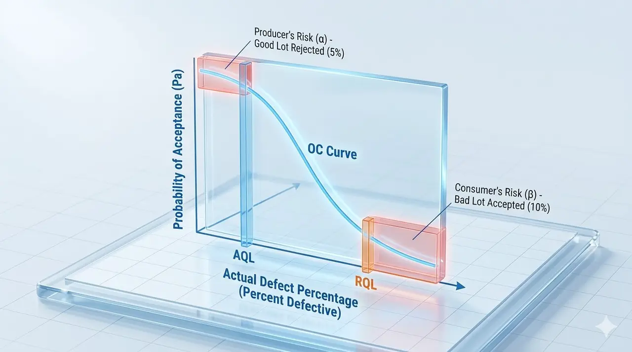
The Operating Characteristic (OC) Curve visualizes the discriminatory power of a sampling plan.

• Y-axis: Probability of Acceptance (Pa).
• X-axis: Actual defect percentage in the lot (Percent Defective).

Manufacturers and buyers use the OC Curve to assess two key risks:

• Producer’s Risk (Alpha): The probability that a good lot (quality equal to or better than AQL) is erroneously rejected. Typically set at 5%.
• Consumer’s Risk (Beta): The probability that a bad lot (quality worse than RQL/LTPD) is erroneously accepted. Typically set at 10%.

How to Use AQL Tables (ISO 2859-1)

AQL tables, also known as AQL charts, are the standardized tools based on ISO 2859 that inspectors and quality managers use to execute the sampling process. They provide a simple, systematic way to determine the appropriate sample size for an inspection and the specific number of defects that are acceptable for a given batch size and AQL. The process involves two primary tables.

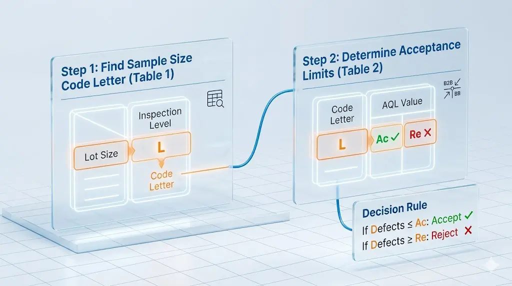
Step 1: Find the Sample Size Code Letter (Table 1)

Locate the row corresponding to the Lot Size (total quantity) and the column for the chosen Inspection Level (e.g., General Level II). The intersection provides a Code Letter (e.g., A, B… M, N).

Step 2: Determine Acceptance Limits (Table 2)

Locate the row for the Code Letter in Table 2. This row defines Sample Size (n). Move across to the column matching the agreed AQL (e.g., 2.5). This cell provides:

• Acceptance Number (Ac): Maximum allowable defects.
• Rejection Number (Re): Threshold for rejecting the batch.
• Decision Rule: If defects found are less than or equal to Ac, accept. If defects are equal to or greater than Re, reject.

Example Scenario

Context: An electronics retailer places an order for 10,000 phone chargers from a factory. To ensure quality without checking every unit, the retailer’s Quality Control team agrees to perform a Pre-Shipment Inspection (PSI) using the industry standard General Inspection Level II. They establish an AQL of 2.5 for major defects (functional failures like not charging) to balance risk and cost.

Calculation Process:

• Table 1: The inspector locates the lot size range 3,201 to 10,000. Crossing this row with the column for Level II, they identify the Code Letter L.
• Table 2: Referring to Row L, the table specifies a sample size of 200 units.
• Limits: The inspector moves across Row L to the column for AQL 2.5. The table displays Ac = 10 and Re = 11.
• Result: The inspector randomly tests 200 chargers.
  • If 10 or fewer are defective: The lot passes.
  • If 11 or more are defective: The lot fails and is rejected.

Best Practices for Implementing AQL

Organizations should follow these guidelines to ensure AQL standards effectively control quality risks.

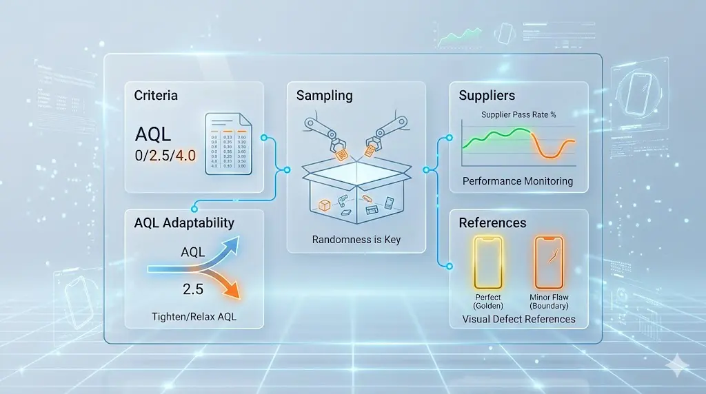
Define Explicit Acceptance Criteria

Do not rely on verbal agreements. Document specific AQL limits (e.g., 0/2.5/4.0) and Defect Classifications (Critical/Major/Minor) in the Purchase Order (PO) or Quality Manual. Ensure suppliers acknowledge these standards before production begins.

Ensure True Random Sampling

Sampling validity depends entirely on randomness. Inspectors must pull samples from all parts of the lot (top, middle, bottom, front, back) rather than just the easiest accessible cartons. Avoid letting factory staff select the samples to prevent bias.

Data-Driven Supplier Management

Use AQL inspection reports to track supplier performance over time.

• Good Performance: If a supplier passes 5 consecutive inspections, consider switching to Level I (Reduced inspection) to save costs.
• Poor Performance: If a supplier fails frequently, switch to Level III (Tightened inspection) or mandate 100% inspection at their expense.

Dynamic AQL Adjustment

AQL standards should evolve. If customer returns increase despite passing PSI (Pre-Shipment Inspection), the current AQL (e.g., 2.5) may be too loose. Tighten the limit (e.g., to 1.5) to filter out more defects. Conversely, if a product is mature and stable, relax the AQL to reduce inspection overhead.

Clear Defect Lists (Golden Samples)

Ambiguity leads to disputes. Provide “Golden Samples” (perfect units) and “Boundary Samples” (marginally acceptable units) to inspectors and factories. This visual reference reduces subjectivity when classifying defects as Major or Minor.

Conclusion

AQL serves as a critical contract between buyers and suppliers, converting subjective quality expectations into objective, quantifiable data. By implementing ISO 2859-1 standards, organizations can streamline inspections, reduce labor costs, and enforce consistent quality limits without the burden of examining every unit. However, inspection alone does not improve quality. To maximize value, businesses must use AQL data not just for batch approval, but as a diagnostic tool to identify production trends, hold suppliers accountable, and drive long-term process improvements.